Effective Train/Test Stratification for Object Detection

September 30, 2022

There’s an unavoidable, inherent difficulty in fine-tuning deep neural networks for specific tasks, which primarily stems from the lack of training data. It would seem ridiculous to a layperson that a pretrained vision model (containing millions of parameters, trained on millions of images) could learn to solve highly specific problems. Therefore, when fine-tuned models do perform well, they seem all the more miraculous. But on the other hand, we also know that it is easier to move from the general to the specific, than the reverse. Specialization after generalization is easier than the reverse.

However, it is this specialization that, when overdone, leads to overfitting. In shallow learning with small data, the problem of overfitting is well understood, and has many solutions like regularization and cross validation, among other things. Further, these methods can be applied independent of whether it is a classification or a regression problem. This is because both the model (a shallow one) and the data (structured, relational) can be reasoned about. Coefficients of linear models, kernel functions and splits of trees have very well studied geometrical interpretations, as do the multivariate statistics of the data itself. In deep networks, however, an equivalent geometrical or statistical reasoning is not for the faint of heart, even if it is possible at all. Not to mention that cross validating deep networks is prohibitively expensive, and regularizing a deep network beyond what its architecture already supports is practically unfeasible (you wouldn’t want to change regularization rates of arbitrary layers in a deep network in the process of fine-tuning, if you can help it).

Ultimately, avoiding overfitting boils down to presenting samples to the model that are most representative of the data which the model is expected to encounter. This is where the disparity between unstructured data like images and text on the one hand, and structured, relational data on the other, becomes very apparent. In the following sections, I’ll discuss the problem of picking representative samples of data in the context of object detection. I’ll propose some methods of fixing this problem, followed by three experiments where I have applied these methods, and their results. (You may choose to skim through the next two somewhat theoretical sections, and skip directly to the examples.)

Stratification in Object Detection

Let us first note that overfitting has many signs - divergence in training and validation loss curves, bad values in class-imbalance metrics, high sensitivity to noise, etc. None of which are solely indicative. Alleviating these individual symptoms may be necessary, but not sufficient to avoid overfitting. For example, simply ensuring that validation error reduces with training error may not be enough. First of all, the divergence between train and validation errors must be interpreted in a relative sense - there is no value of difference between them which may be considered low enough. Secondly, even if the divergence is low, we may still see samples on which the model performs badly - and all we can do is oversample them or augment them.

Examples of this phenomenon crop up routinely in object detection problems. In simpler ML tasks like classification or regression, alleviating a single symptom might be enough. But object detection is a compound problem - it has to identify the “what” and the “where”. Thus, object detection models usually work by minimizing two losses - one for classification of objects, and another for a regression task which locates where an object lies. It is further compounded because the classes are not always mutually exclusive and collectively exhaustive. Given a finite number of classes, any subset of them can occur any number of times in a given image (in fact, it helps to think of this as a word-count distribution in a corpus of text documents - just like any number of words can occur any number of times in document, any number of object classes can occur any number of times in an image). Because of this compounding of label occurrences in a dataset, stratification becomes highly non-trivial.

For instance, consider how we think about stratification in classification tasks. Let’s say that there are primarily three types of classification problems:

Binary classification - each input maps to exactly one of two outputs.
Multiclass classification - each input maps to exactly one of $k$ outputs ($k > 2$)
Multilabel classification - the output is a result of multiple draws from a set $S$ of unique labels with replacement.

It is easy to see that stratification can be readily applied to the first two kinds of problems. In the third case, however, the idea of a representative subset becomes somewhat intangible. Worse, if we throw in regression, then we are left with no straightforward way to classify train/test splits.

At the heart of it, stratification relies on the idea that labels follow some known distribution, and that the train and validation subsets should both be drawn from the same distribution. For the three classification types mentioned above, these distributions are, respectively, Bernoulli, Categorical and Multinomial (or even Dirichlet-multinomial, see the last section).

But for compound problems like object detection, not only can we not pick a distribution apriori, but even if we did, estimating and then sampling it would be too much trouble. (Statistically, the distributions of labels in binary and multiclass classification are univariate, i.e. the sample drawn from the distribution is a scalar. But in multilabel problems, entire vectors have to be drawn from a multivariate distribution.)

So then we’re left with the following hack:

train and evaluate the model on random splits,
find common attributes of samples on which the model produces the greatest loss,
find some way of boosting the model’s performance on the “bad” samples.

The last item here provides the most room for creativity. There are many ways of penalizing the model for specific data samples, including sample-wise weight updates, custom loss functions, etc.

But these methods are not without their challenges. For instance, in object detection, it’s not too useful to attach a weight to an entire image - the model isn’t learning an attribute of the “entire” image at all. It is instead learning attributes of highly localized objects within the image. Similarly, customizing the loss to penalize specific behaviour is a gamble. There’s no way to know whether it will help unless it is accompanied by rigorous experimentation (and if you have the time to do that much work, then fine-tuning an object detection model on a small dataset is perhaps the least of your problems). So our only real choice at this point, is to analyze bad samples in a fully empirical manner, and see how we could have done better. Typically, in object detection, identifying where the model is making the most mistakes translates into identifying classes and sizes of objects that the model usually gets wrong. Most such errors result from some combination of the following effects:

Certain classes of objects are not classified correctly (misclassifications).
Some are not detected at all (false negatives).
The model thinks there are specific types of objects where there are none (false positives).
The model fails to locate objects that are either too small, too large, or some specific size (overfitting or underfitting in the regression part of the model).

We know what to do to alleviate each of these individual problems. They can all be mitigated with better sampling and stratification. But when they all occur together in a single sample (say, an image), a stratification method has to be created. Essentially, when we talk of stratifying a dataset into a train/test split - the question we must first answer is: stratify the data by what?

Attributes of Target Variables

The target vectors for binary and multiclass problems look like this:

y_bin   = [0, 1, 0, 1, 1, 0, 0, 1, ...]
y_multi = [0, 2, 0, 2, 2, 1, 2, 2, ...]

Both of these are easy to interpret, and can be straightaway used for stratification. But here’s what the target (or annotation) of a detection dataset looks like:

[
  {
    "boxes": [
    	[506.97, 352.39, 609.44, 419.26],
    	[446.55, 298.58, 537.16, 363.30],
    	[314.60, 147.72, 640.00, 480.00]
    ],
    "labels": ["bowl", "bowl", "dining table"]
  },
  {
    "boxes": [
    	[36.8300, 113.6800, 601.2200, 396.9000],
    	[105.0400, 167.1500, 271.0600, 293.6500]
    ],
    "labels": ["banana", "apple"]
  }
]

(These are the annotations for a couple of samples from the MS COCO dataset. They tell us that the first image contains two bowls and a dining table, and the second one contains a banana and an apple. It also contains information on where they are in the image.)

If the label $y$ is a simple enough (or univariate) object - like the y_bin and y_multi above - it’s easy to use $y$ for stratification. But how do you stratify a dataset based on a $y$ that has a fairly complex structure, like the one in the second example?

The key idea is,

As a learning task evolves from simple forms like binary or multiclass classification, to complex ones like detection, the variable $y$ acquires additional attributes. Thus, for optimal stratification, most of (if not all of) the available attributes should be leveraged.

Let’s take a deeper look at what this means for two extreme cases.

In binary or multiclass problems, $\mathbf{y}$ only has one attribute, i.e. its membership of some class. $\mathbf{y}$ can itself be interpreted as a single Bernoulli or categorical random variable. In other words, we have a distribution over the training dataset. Given a label $y_i$, this distribution tells us the probability of that label occurring in the dataset.

In detection, however, each target annotation has multiple attributes (the label, the corners of the bounding box, its size, etc), each of which can be random variable in its own right. Looking at the example annotation above, we can define a few of these RVs which capture different attributes of the target:

The RV $X$ = number of objects in the image
The RV $Y$ = average area of the bounding boxes as percentage of the total image size
The RV $Z$ = average distance of the center of a bounding box from the closest image border (is a box closest to the left, right, top or bottom edge? And what’s the distance to that closest edge?)

How are these RVs useful? They’re useful because:

We will want to stratify by $X$, because we don’t want to train on images that have too many objects and validate on images that have too few.
We will want to stratify by $Y$, because we don’t want to train on images that have large objects, and then validate images that have small ones.
We will want to stratify by $Z$, because we don’t want to train on images that are square in the center of the image, and validate on those where objects are along the edges, perhaps only partially captured by the camera.

Now, depending on which of these mistakes the model is making, we could choose which RV to stratify the data by. But we’d be lucky if the model is making only one of these types of mistakes (see the examples below)! It’s common for fine-tuned models to make many different types of mistakes. Each of these RVs represent some aspect of our data. Any of these aspects could end up being underrepresented in our train/test splits! So, we may not have the luxury of stratifying our dataset based on only one RV.

But the good news is that all of these RVs have the same support - the images in dataset. So we can think of the dataset as a joint probability distribution over $X$, $Y$ and $Z$. In other words, we can ask questions like “What is the probability of an image having three objects, such that the average area of them is 200 pixels, and most of the objects are within 5 pixels of the edges?”. This probability can be denoted by $f_{X, Y, Z}(3, 200, 5)$. And when we choose to stratify by this JPD, we are essentially ensuring that the answer to this question does not change between the train and test sets, i.e.

$$ f_{X_{train}, Y_{train}, Z_{train}}(x, y, z) \approx f_{X_{test}, Y_{test}, Z_{test}}(x, y, z) $$

Here we’ve considered only three very specific aspects of object annotations as RVs, and imagined a JPD composed of them. But there’s no rule of thumb about what aspect should be considered a good candidate for stratification. Actually that would depend entirely on what a particular model gets wrong in a particular dataset. Generally, any aspect of a target variable that is quantifiable is a good candidate for adding to the JPD.

In the following section, I describe three different examples, in which I have tried to make this JPD-sampling approach more methodical.

Examples & Illustrations

In order to demonstrate how different stratification strategies can be devised for different problems, I have picked three object detection datasets. For each of them, I have compared the performance of a model trained and validated with a random split, with that of an identical model trained and validated on a stratified split. The datasets range from highly chaotic (varying backgrounds, image sizes, object classes) to somewhat homogenous (fixed camera, a unique background, small number of objects of a similar size, etc). Depending on how chaotic or homogenous a dataset is, we will be able to experiment with different stratification methods.

Common configuration for all experiments

The examples cover three different datasets. The samples are deliberately kept small (upto ~200 images each) for a few reasons:

we want to give the model a hard time, ensuring it extracts the most learning out of a relatively small sample (but not unfairly small)
large datasets of object annotations are anyway hard to come by - they are pretty expensive to create.
a small dataset is easier to visually inspect and debug
the small size takes nothing away from the point I’m trying to make - in fact smaller datasets reinforce it.

For each of the three datasets, we do a total of 40 experiments (a number I picked considering solely my GPU performance and how much time I could spend on a series of experiments). In each such experiment:

we start with a torchvision implementation of Faster-RCNN
do a random 60:40 split of the data
fine-tune the model and collect mAP IoU scores for each image in the test subset.

These scores are collected for all 40 runs and called random split scores.

Then, we select the samples for which the random split score was relatively the worst, and try to identify what the model is failing at. Based on that, we devise stratification strategies, and repeat the 40 experiments - except this time, the split is stratified, not random. We ensure that the no other hyperparameters are different from the random split runs, and that the model runs for the same number of epochs starting from the base model each time. The new group of scores is called the stratified split scores. Now we can compare the two groups of 40 numbers.

For each experiment, we ask

All other things being the same, does stratification alone improve the average mAP IoU? If so, is the improvement statistically significant?

Example 1: Chess Pieces Detection

This dataset contains 202 images of a chess board with pieces. This represents a fairly homogenous dataset, where the images vary in only very few aspects. The orientation of the board and the camera position are mostly fixed. The only variation between the images is the presence and position of different chess pieces.

After the 40 random splits, we see an average mAP IoU of 0.4

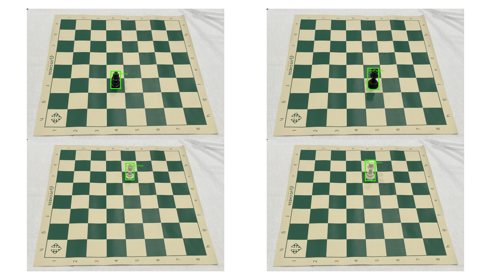
The images that showed the worst metrics had many false negatives, particularly cases of single pieces not being detected. Among those, the model was especially bad at recognizing bishops and queens when they appear by themselves. Given that, it was clear that the data needed to be stratified by how many pieces are present on the board. Surprisingly, this actually decreased the performance by a percent!

However, if we look at the distribution of number of pieces in each image, it turns out that 102 of the 202 images have only one chess piece in them! No surprise, then, that the model gets a few bishops and queens wrong.

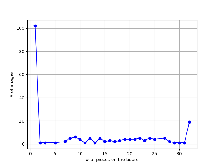
Further, this presents a unique opportunity. Since almost half the images have only one object in them, that subset can be treated as a multiclass problem and stratified simply based on which piece is present in each of those 102 images. The remaining 100 images can then be separately stratified by the total number of pieces in them.

This second strategy yields an improvement of 6%, which is statistically significant. (a one sided T-test with the alternate hypothesis that the stratified split scores are higher, yields a P value of 0.001).

To summarize, this is an example of how we can get somewhat better results with a trivial stratification method, when the data is mostly homogenous.

Example 2: Pedestrian Detection with the Penn-Fudan Dataset

This dataset comes from the torchvision fine-tuning tutorial. It is an instance segmentation dataset, and contains 170 images of pedestrians against roads, sidewalks and crossings. It is significantly more heterogenous than the last dataset, since the image backgrounds vary a lot (pictures taken at different locations) - but that diversity is somewhat tempered by the fact that the task only involves detecting a single type of object (foreground vs background, where the foreground is a pedestrian).

After doing the default 40 runs with the random splits, we get an average mAP IoU of 0.5. Here are 5 of the most problematic images from the dataset:

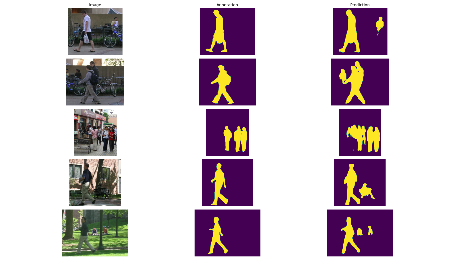
At first glance, it looks like there are many false positives - every image seems to have one or more “central” pedestrians, but the model also picks up many smaller objects all over the image. This suggests that perhaps stratification needs to happen by the size of the annotations (since the image sizes are not fixed, we consider the percentage of the image size that an annotation occupies). But it turns out that stratification by mask size alone does not help at all (it only adds a measly percent to the random split scores).

On digging deeper into the images with bad IoUs, it turns out that the model is greatly overestimating the number of objects. As seen in the image above, the model is quite good at detecting humans - but alas, not all of them are “pedestrians”! In addition, the authors mention that the dataset deliberately ignores occluded objects. So now we add another dimension to the stratification - that of the number of pedestrians in each image.

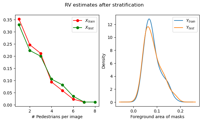
Consider two random variables, $X$ and $Y$ denoting respectively the number of pedestrians per image, and the foreground area occupied by the masks in each image. We need to stratify the dataset by both $X$ and $Y$. It turns out that $X$ and $Y$ can be described with a Poisson and a log-normal distribution quite well. If such distributions are to be found in the annotations, then their JPDs can be helpful in stratifying the data. However, in this case, for the sake of simplicity we still proceed with a purely empirical distribution.

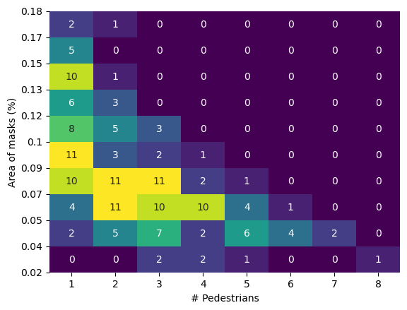
distribution of size and number of pedestrians

Combining $X$ and $Y$ can be done with a 2D histogram as shown above. Each cell in the histogram has a set of images that have the same number of pedestrians, and nearly the same foreground area. Each cell can thus be assigned a unique ID, and that ID can then be used for stratification (Caution: In this case, stratification is not directly possible from the histogram shown above - note that many cells have only one image in them. Do these images go in the train split or the test split? This can be fixed by carefully adjusting bin edges when computing the histogram, such that each cell has at least two images). To see if the stratification has actually worked, we can always estimate the RVs independently in the train and test splits, and see if they match closely enough.

train test distribution of random variables

After performing another 40 runs with this JPD-sampling strategy, the average scores increase to 0.53 - the additional 3% is not statistically significant (we could not reject the null hypothesis of a one sided T-test), but the variance of the stratified split scores is drastically lower - which suggests that the model may be reaching its limits. I still count this as a win, because with the stratification, there is very little uncertainty about how well the model will score. In other words, the model is showing it’s “true” potential.

(On further analysis of the predictions, it turns out that the model is indeed performing much better in a detection sense - it detects humans very well. The mAP IoU scores are low because the model can’t differentiate between humans and pedestrians, and the test labels only care about pedestrians. And indeed, the training data gives us no such differentiation explicitly - it simply ignores humans that are not pedestrians, leading to the large number of false positives in the predictions. Instead of pushing and squeezing the model even harder, it is easier to solve this problem in post-processing of the predictions, such as by non-maximal suppression and morphological operations to eliminate occluded objects.)

Example 3: Subset of MS COCO

The last experiment was performed on 200 random samples from the MS COCO dataset, consisting of eight labels - apple, banana, bowl, broccoli, carrot, cup, dining table and knife. I selected these labels because I was looking for subsets of the images with a common theme (this is a subset of the labels which is likely to occur in kitchens). In the other two datasets we could expect some homogeneity. This dataset lies at the other extreme, even with the label filters I chose. This sample is highly chaotic - objects vary by size, count, even presence. The backgrounds vary too - only a few of the images are actually from a kitchen!

Since, unlike the other datasets, here we have eight classes, the metric needed to be modified a bit - we compute the average mAP of IoU for each class over the test images, and then average them for each image. In the first 40 experiments with random splits, this class-wise averaged metric was 0.3. (This was surprising since the base model is itself trained on COCO! It should have seen each of these 200 images before.)

Looking at the results, it was found that:

The model almost always fails to recognize apples (the rarest class).
It thinks that any flat surface with other objects on it is a dining table (the second most frequent class).
It fails to recognize cups when they are tiny (compared to the image size).

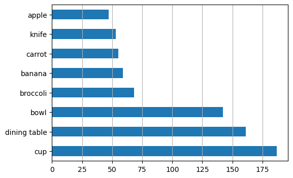
These three are the most frequent and the rarest classes in the dataset. Thus, one way to stratify the dataset would have been by how many apples, dining tables and cups there are in each image. This approach would be a generalization of what we did in the previous example with the RVs $X$ and $Y$ - here we are doing a joint stratification based on three RVs (one for counts of apples, cups and dining tables). But, since the labels were of a Dirichlet-multinomial nature (refer to the word-count analogy I’ve used earlier), I wanted to see if there’s a more methodical way to stratify data of this nature.

If we look solely at the image-wise class count data, it is very tempting to treat the grouping of this data as a topic modeling problem, just like we do for text corpora. LDA, a topic modeling method, posits that there exist latent (abstract or unseen) groups of words. All such groups share a common theme, and are therefore interpreted as “topics”. Natural language texts, then, can be interpret as the effect of mixing words from these topics. Thus, each document in a corpus “belongs” to each topic to some extent. There’s no reason that this analogy could not be applied to a set of images with multiple classes, each of which can occur zero or more times in a single image. Let’s take the analogy a bit further. Suppose, we want to caption each image in our dataset by describing (in English) how many of each type of objects it contains. Now, if we were to apply LDA to these captions (and if it worked well enough), we could assign a topic to each caption, and therefore each image! We then just pick samples from each topic.

However, in a practical sense, LDA needs both a sufficiently large vocabulary (ours only has eight words!) and a sufficiently large corpus of documents (ours only has 200) in order to make sense. So then we fall back to the next best thing that can be done with the label count data: clustering.

If we look for eight clusters (it’s a coincidence that we have eight labels, and the default number of clusters used in sklearn’s implementation of KMeans is also eight) in our label count dataset, we see that each cluster is dominated by a single class.

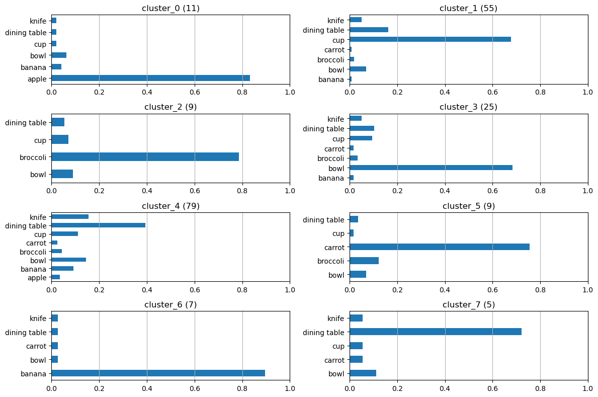
We can now easily draw samples from each of these clusters in a 60:40 ratio, combine them into train and test splits, and that would count as a stratified split. The results from this strategy were no better than the random split. This new model does get most of the cups right (the cluster dominated by cups is one of the largest - they’re sufficiently well represented). But that increase in performance is negated by the model getting sizes of the dining tables thoroughly wrong. The predicted dining tables are either much larger or much smaller than the true boxes. This gives us another hint - so far we have the cluster IDs as one stratification key, maybe we need to look for size distributions of different classes too?

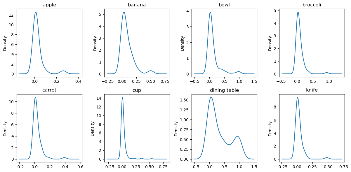
We look at the KDEs of the sizes of different labels in the dataset. And voila! The distribution of the sizes for dining tables is very strongly bimodal! This means that there are mainly two sizes of dining tables in the dataset which can reasonably be called “small tables” and “large tables”. Finally, to compensate the model’s performance with dining table sizes, we can stratify the data by one additional RV, i.e. whether a dining table exists, and if it does, is it small or large?

Stratifying by a joint distribution of the cluster IDs and this additional RV, and repeating the 40 experiments, we get a boost of only 2%, but it is statistically significant. And while the average performance does not increase much (since we’re averaging metrics across classes), the mAP of IoU for dining tables, cups and apples show an increase, albeit at the cost of broccoli and carrots.

(My craft is but a reflection of my self. My model, like me, is apparently blind to healthy food. It’s difficult to feel too bad about broccoli going unnoticed.)

Conclusion: We can do better than random splits, even in computer vision

When training deep networks on unstructured data we generally tend to neglect statistical inference. But we don’t have to leave the poor black box to fend for itself. Curated train/test splits can go a long way in helping the models overcome common pitfalls. None of the stratification methods described above are hard and fast, or even guaranteed to improve performance. Indeed, in one of the three examples, the improvement was not statistically significant. And whatever marginal improvement we saw in the other two was not numerically significant. But note that these experiments have been carried out within very harsh constraints - only ~200 images, only 20-30 epochs, small train:test ratios, no image augmentation, no hyperparameter tuning, etc. We deliberately wanted to squeeze the last bit of performance from the model based on nothing but better train/test splits. If we start relaxing these constraints, the models will only improve.

So why bother, in the first place, with this painful exercise of first identifying aspects of labels that can be modeled with distributions, then combining them into a JPD and then finally sampling from it?

These experiments are only a few illustrations of how stratification can be done more intelligently. These hacks become necessary because sometimes, the limitations on the data and the model are all too real. In these examples, I did want the model to have a hard time. But in most other problems, both my model and I will have a hard time all by ourselves, without anyone imposing additional restrictions.

I have myself said, on many occasions, that hacking around with a model beyond reasonable limits is usually not worth the trouble. This post is for when it is worth the trouble. When they are cornered, a desperate ML researcher will go to any lengths - even if that means taking a sledgehammer to an underground vault and digging out old statistics textbooks.

Acknowledgements: Many thanks to Bhanu K and Shreya Y for reviewing early drafts of this post.

PS: The scripts and notebooks used to run these examples are available here. I apologize for the poorly structured code and lack of documentation - I did not initially write them for others to use. The only reason I am sharing it here is so that I myself don’t misplace it. If you would like to use them in any way, please leave a comment below and I’ll get them ready to use.